Ballot Polling with and without Replacement
Contents
Ballot Polling with and without Replacement#
A martingale approach suggested by the work of Harold Kaplan#
P.B. Stark#
Nonparametric lower confidence bounds for the mean of a non-negative population#
Suppose the real random variable \(X\) has CDF \(F\) and \(\mathbb P \{X \ge 0 \} = 1\). We seek a lower confidence bound for \(\mu \equiv \mathbb E X = \int_0^\infty x dF\).
Under the hypothesis that \(\mu = t\),
Fix \(\gamma \in [0, 1]\). Because \(\int_0^\infty dF = 1\), it follows that if \(\mu = t\),
Now, $\( \mathbb E \left [(\gamma/t) X + (1-\gamma) \right ] \equiv \int_0^\infty \left (x \gamma/t + (1-\gamma) \right ) dF(x). \)\( Since for \)x \ge 0\(, \)(x \gamma/t + (1-\gamma)) \ge 0$, it follows that if we define
then \(G\) is the cdf of a nonnegative random variable.
Let \(Y\) be a random variable with cdf \(G\). By Jensen’s inequality, \(\mathbb E X^2 \ge (\mathbb E X)^2 = t \cdot \mathbb E X\) (by hypothesis). Since \(\mathbb E X = t \ge 0\),
(The penultimate step uses Jensen’s inequality.)
If we reject the hypothesis \(H_0\) that \(X \sim F\) in favor of the alternative hypothesis \(H_1\) that \(X \sim G\), we have evidence that \(\mu = \mathbb E X > t\).
A martingale test for the mean for sampling with replacement#
We observe \(X_1, X_2, \ldots\) IID \(F\). Suppose \(\mathbb{E} X_j = t\). Define
This is a polynomial in \(\gamma\) of degree at most \(n\), with constant term \(1\). Each \(X_j\) appears linearly. Under the null hypothesis that the expected value of \(F\) is \(t\), \(\mathbb{E} X_1 = t\), and
Now
Thus, under the null, $\( \mathbb{E} Y_1 = \frac{\mathbb{E}X_1}{2t} + 1/2 = \frac{t}{2t} + 1/2 = 1. \)$
Also,
Thus, under the null hypothesis, \((Y_j )_{j=1}^N\) is a nonnegative martingale with expected value 1, and Kolmogorov’s inequality implies that for any \(i \in \{1, 2, \ldots, \}\),
Set
and re-write the polynomial
Sampling without replacement#
Let \(S_j \equiv \sum_{k=1}^j X_k\), \(\tilde{S}_j \equiv S_j/N\), and \(\tilde{j} \equiv 1 - (j-1)/N\). Define
This is a polynomial in \(\gamma\) of degree at most \(n\), with constant term \(1\). Each \(X_j\) appears linearly. Under the null hypothesis that the population total is \(Nt\), \(\mathbb{E} X_1 = t\), and
Now
Thus, under the null, $\( \mathbb{E}Y_1 = \frac{\mathbb{E}X_1}{2t} + 1/2 = 1. \)$
Also,
Thus, under the null hypothesis, \((Y_j )_{j=1}^N\) is a nonnegative closed martingale with expected value 1, and Kolmogorov’s inequality implies that for any \(J \in \{1, \ldots, N\}\),
Set
and re-write the polynomial
This expresses the polynomial in terms of its roots, facilitating computations in Python. Using this notation,
Supremum over \(\gamma\) rather than integral over \(\gamma\) (exploration, not proof)#
Let \(S_j \equiv \sum_{k=1}^j X_k\), \(\tilde{S}_j \equiv S_j/N\), and \(\tilde{j} \equiv 1 - (j-1)/N\), as before. Re-define
This is the supremum of a polynomial in \(\gamma\) of degree at most \(n\), with constant term \(1\). Each \(X_j\) appears linearly. Under the null hypothesis that the population total is \(Nt\), \(\mathbb{E} X_1 = t\), and
Now
Thus, under the null, $\( \mathbb{E}Y_1 = t/t + \mathbb{E}Z = 1 + \mathbb{E}Z, \)$
where \(Z \equiv (1-X_1/t)1_{X_1 < t}\). We might be able to construct a submartingale from this if we have an upper bound for \(\mathbb{E}Z\). An upper bound should be pretty straightforward. To be continued…
# First cell with code: set up the Python environment
%matplotlib inline
import matplotlib.pyplot as plt
import math

import numpy as np
from numpy.polynomial import polynomial as P

import scipy as sp
import scipy.stats
from scipy.stats import binom
from scipy.optimize import brentq, minimize_scalar

import random

import pandas as pd

from ipywidgets import interact, interactive, fixed
import ipywidgets as widgets
from IPython.display import clear_output, display, HTML

random.seed(123456789)
Matplotlib is building the font cache using fc-list. This may take a moment.
## Recursive integral from 0 to 1 of a polynomial in terms of its roots

def integral_from_roots(c, maximal=True):
    '''
    Integrate the polynomial \prod_{k=1}^n (x-c_j) from 0 to 1, i.e.,
       \int_0^1 \prod_{k=1}^n (x-c_j) dx
    using a recursive algorithm devised by Steve Evans.

    If maximal == True, finds the maximum of the integrals over lower degrees:
       \max_{1 \le k \le n} \int_0^1 \prod_{j=1}^k (x-c_j) dx

    Input
    ------
    c : array of roots

    Returns
    ------
    the integral or maximum integral and the vector of nested integrals
    '''
    n = len(c)
    a = np.zeros((n+1,n+1))
    a[0,0]=1
    for k in np.arange(n):
        for j in np.arange(n+1):
            a[k+1,j] = -c[k]*((k+1-j)/(k+1))*a[k,j]
            a[k+1,j] += 0 if j==0 else (1-c[k])*(j/(k+1))*a[k,j-1]
    integrals = np.zeros(n)
    for k in np.arange(1,n+1):
        integrals[k-1] = np.sum(a[k,:])/(k+1)
    if maximal:
        integral = np.max(integrals[1:])
    else:
        integral = np.sum(a[n,:])/(n+1)
    return integral, integrals
def HK_ps_se_p(x, N, t, random_order = True):
    '''
    p-value for the hypothesis that the mean of a nonnegative population with
    N elements is t, computed using recursive algorithm devised by Steve Evans.

    The alternative is that the mean is larger than t.
    If the random sample x is in the order in which the sample was drawn, it is
    legitimate to set random_order = True.
    If not, set random_order = False.

    If N = np.inf, treats the sampling as if it is with replacement.
    If N is finite, assumes the sample is drawn without replacement.

    Input:   x, array-like, the sample
    ------   N, int, population size. Use np.inf for sampling with replacement
             t, double, the hypothesized population mean
             random_order, boolean, is the sample in random order?

    Returns: p, double, p-value of the null
    -------  mart_vec, array, martingale as elements are added to the sample


    '''
    x = np.array(x)
    assert all(x >=0),  'Negative value in a nonnegative population!'
    assert len(x) <= N, 'Sample size is larger than the population!'
    assert N > 0,       'Population size not positive!'
    if np.isfinite(N):
        assert N == int(N), 'Non-integer population size!'
    Stilde = (np.insert(np.cumsum(x),0,0)/N)[0:len(x)] # \tilde{S}_{j-1}
    t_minus_Stilde = t - Stilde
    mart_max = 1
    mart_vec = np.ones_like(x, dtype=np.float)
    if any(t_minus_Stilde < 0): # sample total exceeds hypothesized population total
        mart_max = np.inf
    else:
        jtilde = 1 - np.array(list(range(len(x))))/N
        c = np.multiply(x, np.divide(jtilde, t_minus_Stilde))-1
        r = -np.array([1/cc for cc in c[0:len(x)+1] if cc != 0]) # roots
        Y_norm = np.cumprod(np.array([cc for cc in c[0:len(x)+1] if cc != 0])) # mult constant
        integral, integrals = integral_from_roots(r, maximal = False)
        mart_vec = np.multiply(Y_norm,integrals)
        mart_max = max(mart_vec) if random_order else mart_vec[-1]
    p = min(1/mart_max,1)
    return p, mart_vec
## find minimum possible sample sizes to attain significance level alpha
bonfac = 9
for i in range(40):
    p = HK_ps_se_p(np.ones(i+1), np.inf, 0.5, random_order = True)[0]
    print(i+1, p, bonfac*p )
1 0.6666666666666666 6.0
2 0.42857142857142855 3.8571428571428568
3 0.26666666666666666 2.4
4 0.16129032258064516 1.4516129032258065
5 0.09523809523809523 0.8571428571428571
6 0.05511811023622047 0.49606299212598426
7 0.03137254901960784 0.2823529411764706
8 0.01761252446183953 0.15851272015655576
9 0.009775171065493646 0.08797653958944282
10 0.00537371763556424 0.04836345872007816
11 0.0029304029304029304 0.026373626373626374
12 0.001587107801245269 0.014283970211207421
13 0.0008545443447476042 0.007690899102728438
14 0.0004577776421399579 0.004119998779259621
15 0.00024414435034714275 0.0021972991531242847
16 0.0001297006965690351 0.0011673062691213158
17 6.866481271672331e-05 0.0006179833144505098
18 3.6239693145166674e-05 0.00032615723830650006
19 1.9073504518036383e-05 0.00017166154066232744
20 1.0013585097115086e-05 9.012226587403578e-05
21 5.245209990789888e-06 4.720688991710899e-05
22 2.741813986517666e-06 2.4676325878658997e-05
23 1.4305115598745084e-06 1.2874604038870575e-05
24 7.450580818968439e-07 6.705522737071596e-06
25 3.8743019681319884e-07 3.4868717713187895e-06
26 2.0116567761574444e-07 1.8104910985417e-06
27 1.0430812874551165e-07 9.387731587096049e-07
28 5.4016709428311716e-08 4.861503848548054e-07
29 2.7939677264485208e-08 2.5145709538036687e-07
30 1.443549991326197e-08 1.2991949921935773e-07
31 7.450580598658552e-09 6.705522538792696e-08
32 3.841705620736082e-09 3.457535058662474e-08
33 1.9790604711730883e-09 1.7811544240557795e-08
34 1.0186340660153258e-09 9.167706594137932e-09
35 5.2386894822883e-10 4.71482053405947e-09
36 2.692104317267455e-10 2.4228938855407097e-09
37 1.3824319466998802e-10 1.2441887520298922e-09
38 7.094058673841744e-11 6.38465280645757e-10
39 3.6379788070950217e-11 3.2741809263855195e-10
40 1.8644641386353507e-11 1.6780177247718157e-10
def min_p(x, N, t, random_order = True):
    '''
    (putative) p-value for the hypothesis that the mean of a nonnegative population with
    N elements is t, computed assuming it is legitimate to minimize over \gamma --- which
    has not been proven.

    The alternative is that the mean is larger than t.
    If the random sample x is in the order in which the sample was drawn, it is
    legitimate to set random_order = True.
    If not, set random_order = False.

    If N = np.inf, treats the sampling as if it is with replacement.
    If N is finite, assumes the sample is drawn without replacement.

    Input:   x, array-like, the sample
    ------   N, int, population size. Use np.inf for sampling with replacement
             t, double, the hypothesized population mean
             random_order, boolean, is the sample in random order?

    Returns: p, double, p-value of the null
    -------  mart_vec, array, martingale as elements are added to the sample


    '''
    x = np.array(x)
    assert all(x >=0),  'Negative value in a nonnegative population!'
    assert len(x) <= N, 'Sample size is larger than the population!'
    assert N > 0,       'Population size not positive!'
    if np.isfinite(N):
        assert N == int(N), 'Non-integer population size!'
    Stilde = (np.insert(np.cumsum(x),0,0)/N)[0:len(x)] # \tilde{S}_{j-1}
    t_minus_Stilde = t - Stilde
    mart_max = 1
    mart_vec = np.ones_like(x, dtype=np.float)
    if any(t_minus_Stilde < 0): # sample total exceeds hypothesized population total
        mart_max = np.inf
    else:
        jtilde = 1 - np.array(list(range(len(x))))/N
        for j in range(len(x)):
            # use logarithm
            f = lambda g: -np.sum(np.log(g*(x[0:j]/t-1)+1))
            res = minimize_scalar(f, bounds=(0, 1), method='bounded')
            if res.success:
                mart_vec[j] = np.exp(-res.fun)
            else:
                print("minimize_scalar failed", res)
        mart_max = max(mart_vec) if random_order else mart_vec[-1]
    p = min(1/mart_max,1)
    return p, mart_vec
“maximum” KMart#
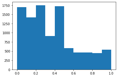
The simulation below shows that a naive use of the maximum over \(\gamma\) does not work: the resulting putative \(p\)-values are stochastically too small.
What remains to explore is whether this can be compensated for by bounding the expectation of the maximum of the product over \(\gamma\).
reps = int(10**4)
p = 0.05
N = 1000
x = [0]*int(N/2) + [1]*int(N/2)
t = np.mean(x)
print('population mean ', t)
t_0 = t
ps = np.zeros(reps)
reject = 0
for i in range(reps):
    np.random.shuffle(x)
    p_min, mart_min = min_p(x, N, t_0, random_order=True)
    ps[i] = p_min
    if i % 500 == 0:
        print('iteration ', i, 'mean p', np.mean(ps[:i+1]))
plt.hist(ps)
population mean  0.5
iteration  0 mean p 0.0036490151493502867
iteration  500 mean p 0.3863844802890874
iteration  1000 mean p 0.37672556237907606
iteration  1500 mean p 0.3725053163978612
iteration  2000 mean p 0.37285394193952426
iteration  2500 mean p 0.37276013517440276
iteration  3000 mean p 0.3727135812680586
iteration  3500 mean p 0.37179283663048174
iteration  4000 mean p 0.3730550116422361
iteration  4500 mean p 0.3742452948059613
iteration  5000 mean p 0.3750336491853684
iteration  5500 mean p 0.3746402810978351
iteration  6000 mean p 0.3731493705366741
iteration  6500 mean p 0.37239843354890867
iteration  7000 mean p 0.3728719798895219
iteration  7500 mean p 0.3730286668500974
iteration  8000 mean p 0.3727155260707411
iteration  8500 mean p 0.3732505816511243
iteration  9000 mean p 0.37273007904308925
iteration  9500 mean p 0.3723466426465058
(array([1701., 1419., 1750.,  915., 1720.,  585.,  460.,  465.,  444.,
         541.]),
 array([2.22363360e-05, 1.00020013e-01, 2.00017789e-01, 3.00015565e-01,
        4.00013342e-01, 5.00011118e-01, 6.00008895e-01, 7.00006671e-01,
        8.00004447e-01, 9.00002224e-01, 1.00000000e+00]),
 <a list of 10 Patch objects>)
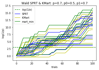
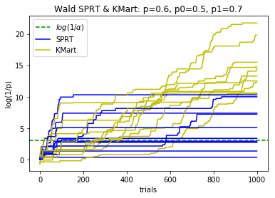
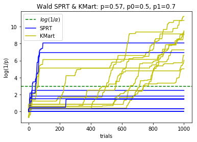
def plotBinomialSPRT(n, p, p0, p1, alpha, reps=10):
    '''
       Plots the progress of the SPRT for n iid Bernoulli trials with probabiity p
       of success, for testing the hypothesis that p=p0 against the hypothesis p=p1
       with significance level alpha.
       Compares with the Kaplan martingale approach that doesn't use the alternative
       hypothesis, and with the maximum over gamma

       Input:
       ------
            n      int, number of trials
            p      double, actual probability of success in each trial
            p0     double, probability of success under the null hypothesis
            p1     double, probability of success under the alternative (SPRT only)
            alpha  double, significance level
            reps   int, number of replications
    '''
    fig, ax = plt.subplots(nrows=1, ncols=1, sharex=True)
    ax.set_title('Wald SPRT & KMart: p='
                + str(p) + ', p0=' + str(p0) + ', p1=' + str(p1))
    ax.axhline(y=math.log(1/alpha), xmin=0, xmax=n, color='g', linestyle="--",
              label=r'$log(1/\alpha)$')
    ax.set_ylabel('log(1/p)')
    ax.set_xlabel('trials')
    for r in range(reps):
        trials = sp.stats.binom.rvs(1, p, size=n+1)  # leave room to start at 1
        terms = np.ones(n+1)
        sfac = p1/p0
        ffac = (1.0-p1)/(1.0-p0)
        terms[trials == 1.0] = sfac
        terms[trials == 0.0] = ffac
        terms[0] = 1.0
        logterms = np.log(terms)
    #
        p_mart, mart_vec = HK_ps_se_p(trials, np.inf, p0)
        p_min, mart_min = min_p(trials, np.inf, p0)
        log_mart_vec = np.log(mart_vec)
        log_mart_min = np.log(mart_min)
        if r < reps-1:
            ax.plot(range(n+1),np.maximum.accumulate(np.cumsum(logterms)), color='b',\
                linestyle='-')
            ax.plot(range(n+1), np.maximum.accumulate(log_mart_vec), color='y',\
                linestyle='-')
            ax.plot(range(n+1), np.maximum.accumulate(log_mart_min), color='g',\
                linestyle='-')
        else:
            ax.plot(range(n+1),np.maximum.accumulate(np.cumsum(logterms)), color='b',\
                linestyle='-', label=r'SPRT')
            ax.plot(range(n+1), np.maximum.accumulate(log_mart_vec), color='y',\
                linestyle='-', label=r'KMart')
            ax.plot(range(n+1), np.maximum.accumulate(log_mart_min), color='g',\
                linestyle='-', label=r'mart_min')
    ax.legend(loc='best')
    plt.show()
plotBinomialSPRT(100, .7, .5, .7, .05)
plotBinomialSPRT(1000, .6, .5, .7, .05)
plotBinomialSPRT(1000, .57, .5, .7, .05)
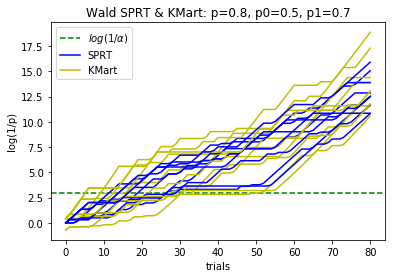
plotBinomialSPRT(80, .8, .5, .7, .05)
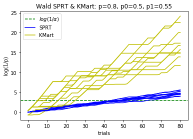
plotBinomialSPRT(80, .8, .5, .55, .05)
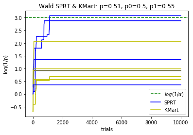
plotBinomialSPRT(10000, .51, .5, .55, .05, reps=5)
Power simulations#
reps = 1000
alpha = 0.05
sam_fac = 10
margins = [0.7, 0.6] # , 0.55, 0.52, 0.51, 0.505]
results = {}
for p in margins:
    results[str(p)] = np.ones(reps)
    n = math.ceil(sam_fac/(2*(p-1/2))**2)  # estimate of a high percentile of the sample size
    for r in range(reps):
        trials = sp.stats.binom.rvs(1, p, size=n)
        p_mart, mart_vec = HK_ps_se_p(trials, np.inf, 0.5)
        mart_vec = np.maximum.accumulate(mart_vec)
        inx = np.argwhere(mart_vec >= 1/alpha)
        results[str(p)][r] = np.min(inx) if inx.size > 0 else n
    print(p, inx.size, n)
0.7 0 63
0.6 0 251
Ballot-polling without replacement, more than two kinds of votes#
We have an election with \(N\) ballots cast for some number of candidates. Some of the ballots might have undervotes or be invalid.
The social choice function considered here is plurality, either vote for 1 or vote for \(k\). Majority and super-majority are easy generalizations.
The candidates \(w \in \mathcal W\) were reported to have beaten the candidates \(\ell \in \mathcal L\). If, for every pair \(w \in \mathcal W\), \(\ell \in \mathcal L\), we can reject the hypothesis that \(w\) received no more votes than \(\ell\) at level \(\alpha\), we have confirmed the outcome at risk limit \(\alpha\).
In a stratified audit, we might need evidence that in a stratum, \(w\) got more votes than \(\ell\) did, plus an additional margin \(c\). The derivation below includes that more general case.
In general, some ballots will have invalid votes or votes for candidates other than \(w\) and \(\ell\). Consider a single pair of candidates \(w \in \mathcal W\), \(\ell \in \mathcal L\). Let \(N_w\) denote the number of ballots in the population that show a vote for \(w\) but not for \(\ell\); let \(N_\ell\) denote the number of ballots in the population that show a vote for \(\ell\) but not for \(w\), and let \(N_u \equiv N - N_w - N_\ell\) denote the number of ballots that show a vote for neither \(w\) nor \(\ell\) or show votes for both \(w\) and \(\ell\).
We sample sequentially, without replacement.
Let \(X_i\) be the label of the item selected on the \(i\)th draw. Let \(W_i\) be the number of items labeled \(w\) selected on or before draw \(i\); and define \(L_i\) and \(U_i\) analogously. The probability distributions of those four variables depend on \(N_w\), \(N_\ell\), and \(N_u\), even though we only care about one parameter, \(N_w - N_\ell\). Now \(N_w \le N_\ell + c\) if and only if \(N_w + N_u/2 \le N_\ell + N_u/2 + c\), and \(N_\ell + N_u/2 = N - (N_w + N_u/2)\), so
Let $\( \mu = \frac{1 \times N_w + \frac{1}{2} \times N_u + 0 \times N_\ell}{N}. \)\( This is the mean of a population derived from re-labeling each vote for \)w\( as 1, each vote for \)\ell\( as 0, and the rest as \)1/2\(. We can test the hypothesis \)\mu \le (1+c/N)/2\( using the same martingale approaches above by simply treating the sampled ballots that way: every ballot with a vote for \)w\( (but not \)\ell\() counts as 1, every ballot with a vote for \)\ell\( (but not for \)w\() counts as 0, and invalid ballots, ballots with votes for other candidates, and ballots with votes for both \)w\( and \)\ell$ count as 1/2.
## Simulations for finite populations
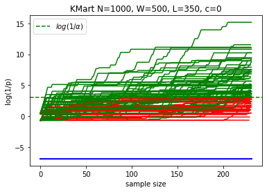
def plotKMart(N, W, L, n, reps=100, c=0, alpha=0.05):
'''
Plots the progress of the Kaplan Martingale and estimates power for a given
sample size
Input: N: population size
W: votes for w
L: votes for l
n: sample size
reps: number of experiments
c: margin required
alpha: risk limit
'''
fig, ax = plt.subplots(nrows=1, ncols=1, sharex=True)
ax.set_title('KMart N=' + str(N) + ', W=' + str(W) + ', L=' +\
str(L) + ', c=' + str(c))
ax.axhline(y=math.log(1/alpha), xmin=0, xmax=n, color='g', linestyle="--",
label=r'$log(1/\alpha)$')
ax.set_ylabel('log(1/p)')
ax.set_xlabel('sample size')
ax.legend(loc='best')
scrambled = [1]*W + [0]*L + [0.5]*(N-W-L)
reject = 0
for j in range(reps):
np.random.shuffle(scrambled)
p_mart, mart_vec = HK_ps_se_p(scrambled[0:n], N, (1+c/N)/2)
log_mart_vec = np.log(mart_vec)
col = 'r'
if np.max(log_mart_vec) >= math.log(1/alpha):
col = 'g'
reject += 1
ax.plot(range(len(log_mart_vec)), np.maximum.accumulate(log_mart_vec), \
color=col, linestyle='-', label=r'Kaplan')
plt.show()
print('margin: ' + str(100*(W-L)/N) + '%, power at sample ' + str(n) + ": " +\
str(100*reject/reps) + '%')
N = 1000
W = 500
L = 350
n = 232 # expected sample size for BRAVO for N=1000, W=500, L=350
reps = 100
plotKMart(N, W, L, n, reps)
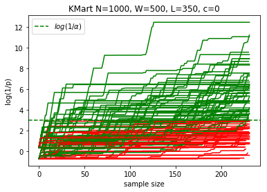
margin: 15.0%, power at sample 232: 59.0%
N = 1000
W = 400
L = 350
n = 300
reps = 100
plotKMart(N, W, L, n, reps)
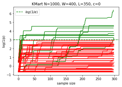
margin: 5.0%, power at sample 300: 11.0%
N = 10000
W = 500
L = 350
n = 1000
reps = 100
plotKMart(N, W, L, n, reps)
/anaconda/lib/python3.6/site-packages/ipykernel_launcher.py:25: RuntimeWarning: overflow encountered in double_scalars
/anaconda/lib/python3.6/site-packages/ipykernel_launcher.py:26: RuntimeWarning: overflow encountered in double_scalars
/anaconda/lib/python3.6/site-packages/ipykernel_launcher.py:26: RuntimeWarning: invalid value encountered in double_scalars
/anaconda/lib/python3.6/site-packages/ipykernel_launcher.py:42: RuntimeWarning: invalid value encountered in multiply
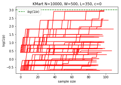
margin: 1.5%, power at sample 1000: 0.0%
Another martingale suggested by S.N. Evans#
We sample sequentially without replacement. Let \(X_k\) be the value of the item selected in the \(k\)th draw, \(k = 1, \ldots, N\). Let \(S_k \equiv \sum_{j=1}^k X_j\).
Define $\( M_k \equiv \begin{cases} \frac{1}{N-k} \frac{S_N - S_k} {S_N},& 1 \le k \le N-1,\\ \frac{X_N}{S_N},& k = N.\\ \end{cases} \)$ This is a margingale.
Define $\( M_k(t) \equiv \begin{cases} \frac{1}{N-k} \left ( 1-\frac{S_k}{Nt} \right ),& 1 \le k \le N-1,\\ \frac{X_N}{Nt},& k = N.\\ \end{cases} \)\( Then if \)t\( is the population mean, \)M_k(t)$ is a martingale, and
def SE_p(x, N, t, random_order = True):
    '''
    p-value for the hypothesis that the mean of a nonnegative population with
    N elements is t, for martingale suggested by Steve Evans.

    The alternative is that the mean is larger than t.
    If the random sample x is in the order in which the sample was drawn, it is
    legitimate to set random_order = True.
    If not, set random_order = False.

    Input:   x, array-like, the sample
    ------   N, int, population size. Use np.inf for sampling with replacement
             t, double, the hypothesized population mean
             random_order, boolean, is the sample in random order?

    Returns: p, double, p-value of the null
    -------  mart_vec, array, martingale as elements are added to the sample


    '''
    x = np.array(x)
    assert all(x >=0),  'Negative value in a nonnegative population!'
    assert len(x) <= N, 'Sample size is larger than the population!'
    assert N > 0,       'Population size not positive!'
    if np.isfinite(N):
        assert N == int(N), 'Non-integer population size!'
    Sk = 1 - np.cumsum(x)/(N*t)
    Nminusk = N-np.array(np.arange(1,len(x)+1))
    MkP = np.divide(Nminusk,Sk)
    print(Sk)
    mart_vec = 1/MkP
    mart_max = 1
    if any(Sk < 0): # sample total exceeds hypothesized population total
        p = 0
    else:
        p = min(MkP) if random_order else MkP[-1]
    return p, mart_vec
x = np.array([1, 1, 1, 0])
SE_p(x, 100, 10)
[0.999 0.998 0.997 0.997] [99 98 97 96]
(96.2888665997994, array([0.01009091, 0.01018367, 0.01027835, 0.01038542]))
def plotKMart2(N, W, L, n, reps=100, c=0, alpha=0.05):
    '''
       Plots the progress of the Kaplan martingale and the Evans and estimates power for a given
       sample size

       Input:   N: population size
                W: votes for w
                L: votes for l
                n: sample size
                reps: number of experiments
                c: margin required
                alpha: risk limit
    '''
    fig, ax = plt.subplots(nrows=1, ncols=1, sharex=True)
    ax.set_title('KMart N=' + str(N) + ', W=' + str(W) + ', L=' +\
                 str(L) + ', c=' + str(c))
    ax.axhline(y=math.log(1/alpha), xmin=0, xmax=n, color='g', linestyle="--",
                   label=r'$log(1/\alpha)$')
    ax.set_ylabel('log(1/p)')
    ax.set_xlabel('sample size')
    ax.legend(loc='best')
    scrambled = [1]*W + [0]*L + [0.5]*(N-W-L)
    rejectK = 0
    rejectS = 0
    for j in range(reps):
        np.random.shuffle(scrambled)
        p_martK, mart_vecK = HK_ps_se_p(scrambled[0:n], N, (1+c/N)/2)
        p_martS, mart_vecS = SE_p(scrambled[0:n], N, (1+c/N)/2)
        log_mart_vecK = np.log(mart_vecK)
        log_mart_vecS = np.log(mart_vecS)
        colK = 'r'
        colS = 'b'
        if np.max(log_mart_vecK) >= math.log(1/alpha):
            colK = 'g'
            rejectK += 1
        if np.max(log_mart_vecS) >= math.log(1/alpha):
            colS = 'y'
            rejectS += 1
        ax.plot(range(len(log_mart_vecK)), np.maximum.accumulate(log_mart_vecK), \
                color=colK, linestyle='-', label=r'Kaplan')
        ax.plot(range(len(log_mart_vecS)), np.maximum.accumulate(log_mart_vecS), \
                color=colS, linestyle='-', label=r'Evans')
    plt.show()
    print('margin: ' + str(100*(W-L)/N) + '%, power at sample ' + str(n) + " Kaplan: " +\
          str(100*rejectK/reps) + '%; Evans:' + str(100*rejectK/reps) + '%')
N = 1000
W = 500
L = 350
n = 232 # expected sample size for BRAVO for N=1000, W=500, L=350
reps = 100
plotKMart2(N, W, L, n, reps)
margin: 15.0%, power at sample 232 Kaplan: 66.0%; Evans:66.0%